How to use VLOOKUP in Microsoft Excel

In Microsoft Excel, VLOOKUP (vertical lookup) is a search function that you lot can employ to observe whatsoever data inside a particular column of the table by looking at the starting time column'southward entries and returning a corresponding value from some other column.

While in a small tabular array, you lot may be able to glance and rapidly determine the information you need, it'due south different when working with an extensive spreadsheet with hundreds of rows and columns. Since you tin spend a long time analyzing and finding the required information, Excel's VLOOKUP office was created to simplify data retrieval.

VLOOKUP works by performing a vertical search (meridian to bottom) for a value in the offset column (that acts as the unique identifier), and and then it returns a upshot from the matching row. The Excel role works like a drink carte at the coffee shop, where you start with the information you know, such as the drink's name, and then you wait to the right to get the information you lot don't know, for example, the price.

In this Windows ten guide, we'll walk you through the steps to correctly write a basic VLOOKUP function with the desktop version of Microsoft Excel, whether you use the version of Office bachelor through a Microsoft 365 subscription, Office 2022, Office 2022, or earlier version.

How to write VLOOKUP function in Excel
How to build VLOOKUP function in Excel

How to write VLOOKUP role in Excel

To write a VLOOKUP function manually in Excel, employ these steps:

Open Excel.
Create the first column with items that volition work equally unique identifiers (required).

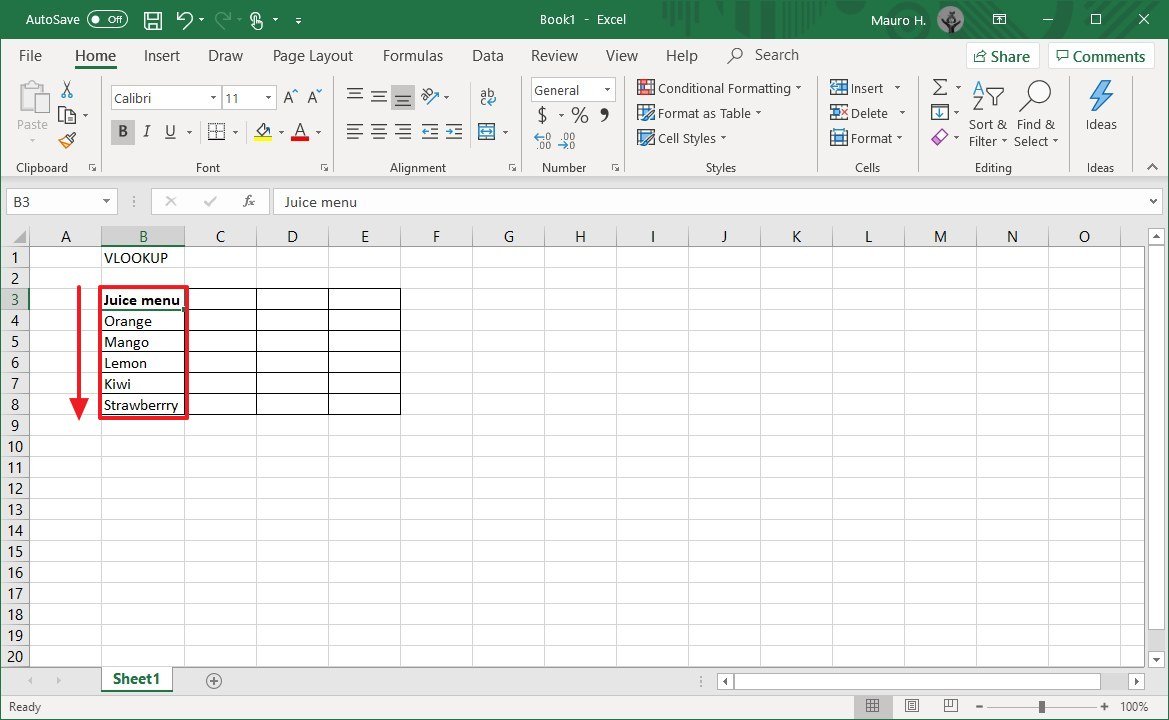Source: Windows Fundamental
Create i or more additional columns (on the right side) with the different values for each item from the first column (on the left side).

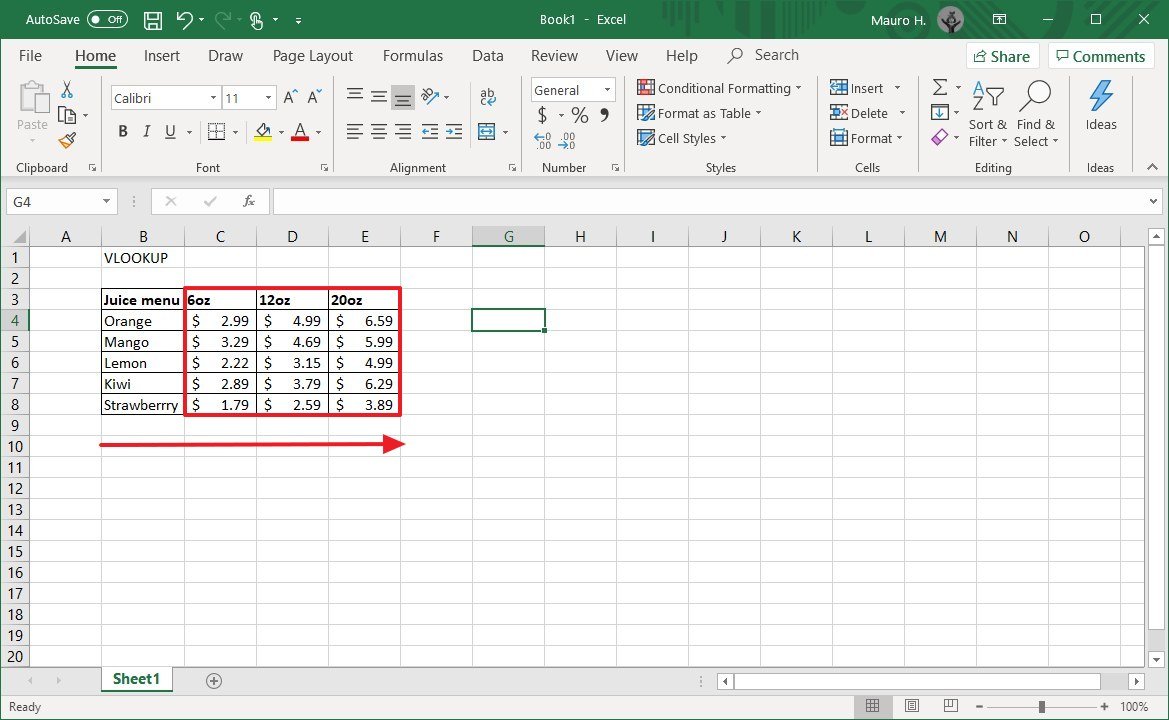Source: Windows Central
Select an empty cell in the spreadsheet and specify the proper noun of the item you want to find an answer to—for example, Orange.

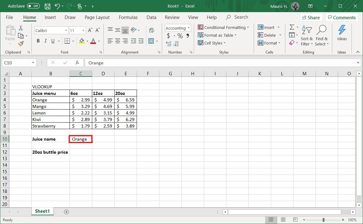Source: Windows Central
Select an empty cell to shop the formula and returned value.
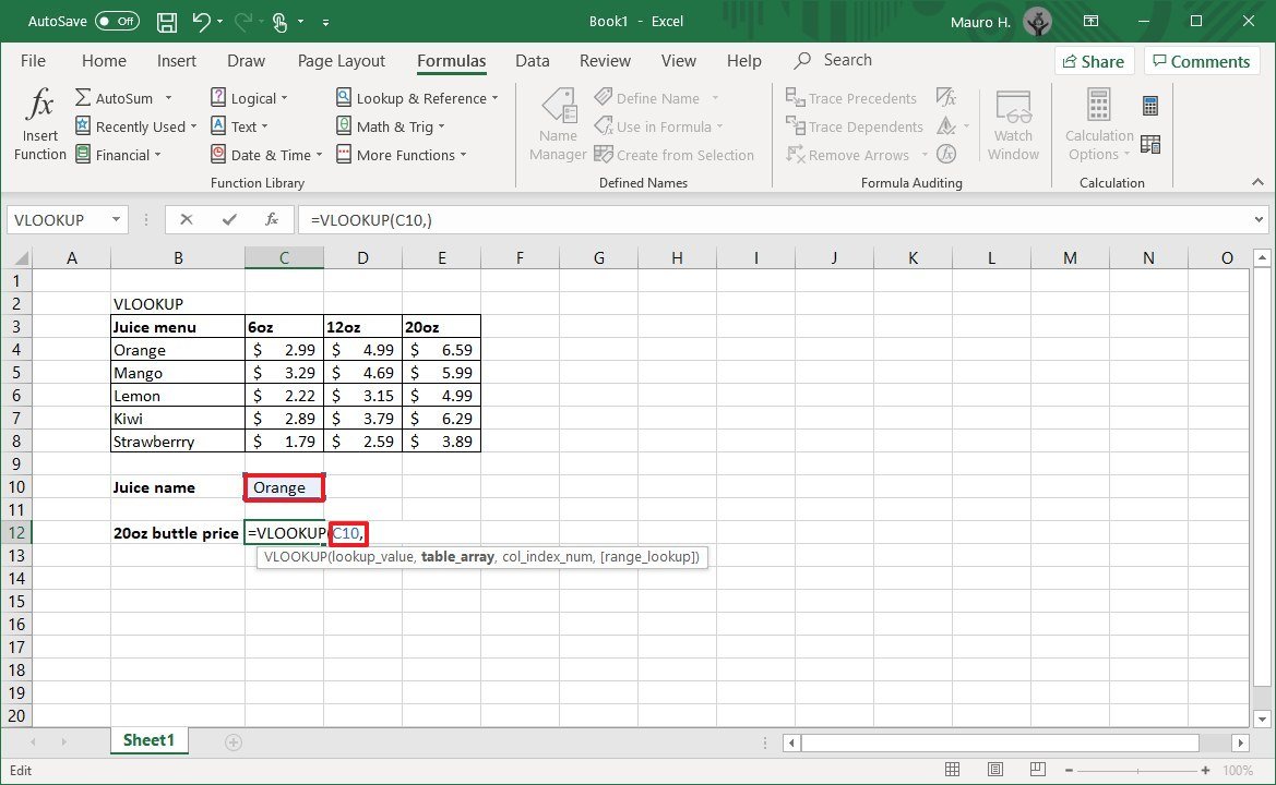
In the empty cell, type the following syntax to create a VLOOKUP formula and printing Enter:

=VLOOKUP()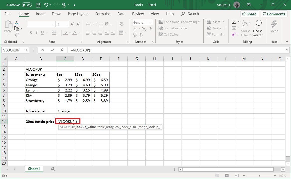

Source: Windows Central
Type the following arguments within the parenthesis "()" to write the function and press Enter:

=VLOOKUP(lookup_value,table_array,col_index_num,range_lookkup)
- lookup_value: defines the cell that includes the product identifier from the first cavalcade on the left.
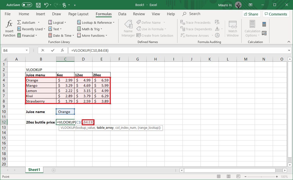
- table_array: defines the range of data where you desire to perform a search. Typically, you would select the unabridged Excel table.
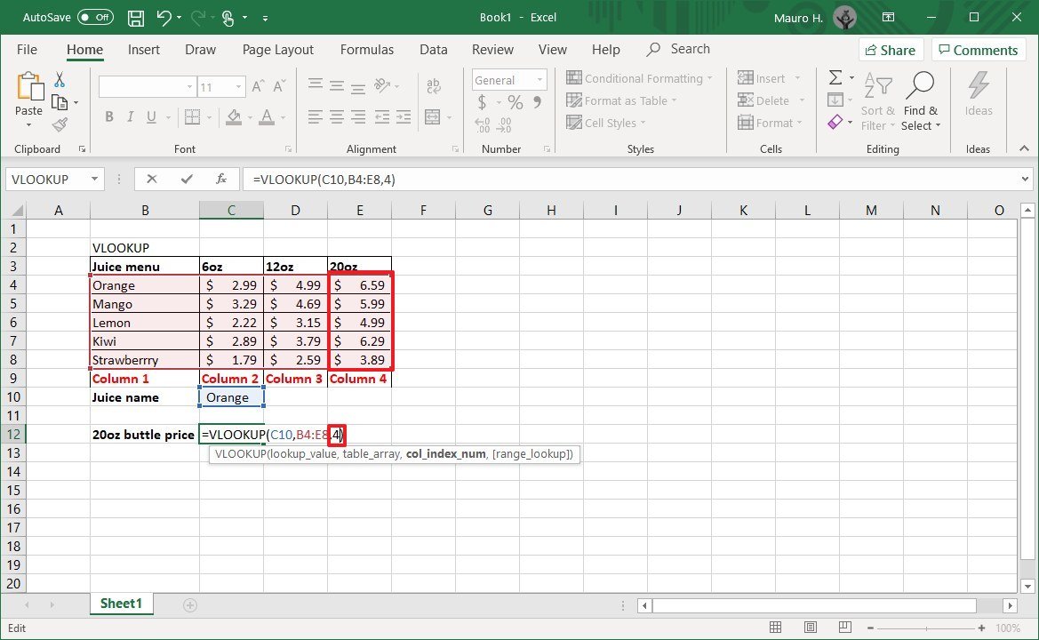
- col_index_num: defines the column number that the part will expect to find a value. When specifying multiple columns, you should do from left to right.
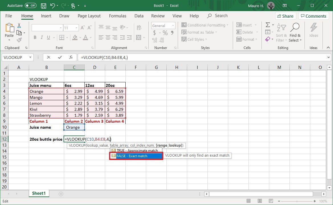
- range_lookkup: includes two options: "false" for exact match or "true" for an judge match. Unremarkably, you want to use the imitation option. Source: Windows Central
  
  Quick note: If yous don't specify a value, then the "true" option volition be applied by default. Sometimes, when using the "truthful" selection, the outset column needs to be shorted, which may cause an unexpected outcome. If yous're not getting the correct value, you should utilise the "imitation" pick or sort the offset column alphabetically or numerically.
In the control, brand certain to update the variables within the parenthesis with the data you lot want to query. Also, remember to use a comma to separate each value in the function. You exercise not need a space between each comma.

Hither's an instance that returns the price for the 20oz bottle of orange juice:

=VLOOKUP(C10,B4:E8,four,Faux)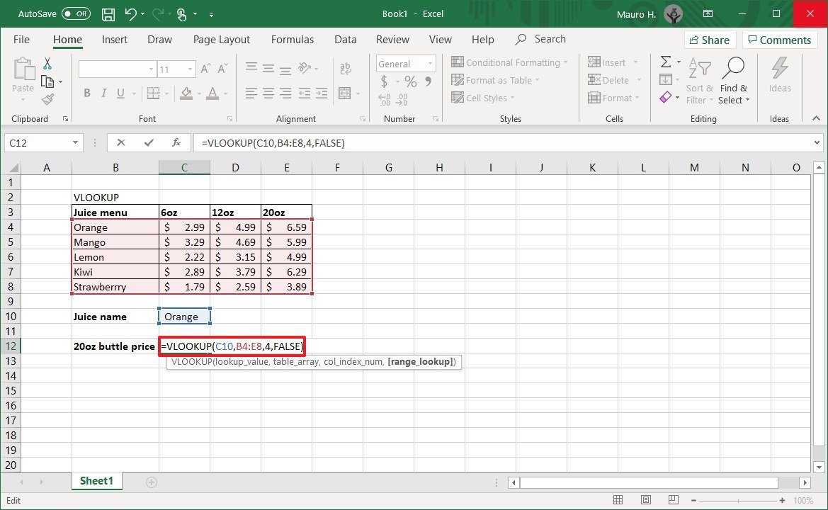

Source: Windows Central

In one case you complete the steps, the feature will return the value for the item you specified on stride No. 4. If you receive the "#Proper name?" error value, then it means that the formula is missing ane or multiple quotes.

If you are trying to find data for another item, update the name of the cell on step No. 4. For instance, if you want to see the price for the "20oz" bottle of Kiwi juice, and so supersede "Orangish" with "Kiwi" in the "lookup_value" cell and printing Enter to update the consequence.

How to build VLOOKUP part in Excel

In addition to writing a formula directly into the spreadsheet, y'all can likewise apply the Functions Arguments sorcerer, which gives you a more convenient interface to build the lookup formula.

To use the Function Arguments wizard to build a VLOOKUP formula in Microsoft Excel, use these steps:

Open Excel.
Create the first cavalcade with a listing of items that will act as unique identifiers (required).

Source: Windows Central
Create one or more than additional columns (on the right side) with the unlike values for each item from the first column (on the left side).

Source: Windows Central
Select an empty cell in the spreadsheet and specify the name of the item you desire to discover an respond to—for case, Orange.

Source: Windows Central
Select an empty cell to store the formula and the returned value.
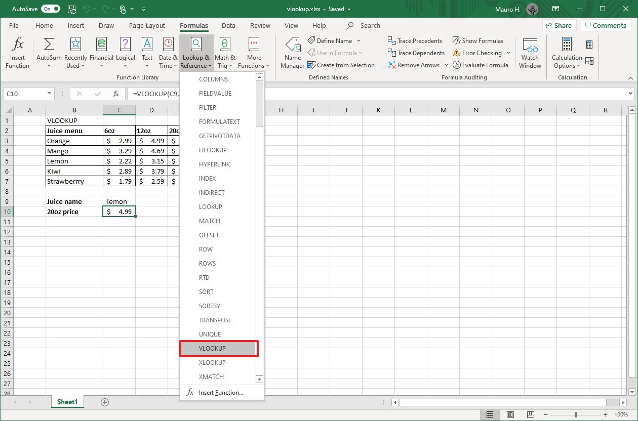
Click the Formulas tab.
Under the "Functions Library" department, click the Lookup and Reference driblet-down menu and select the VLOOKUP option to open up the Functions Arguments wizard.

Source: Windows Central
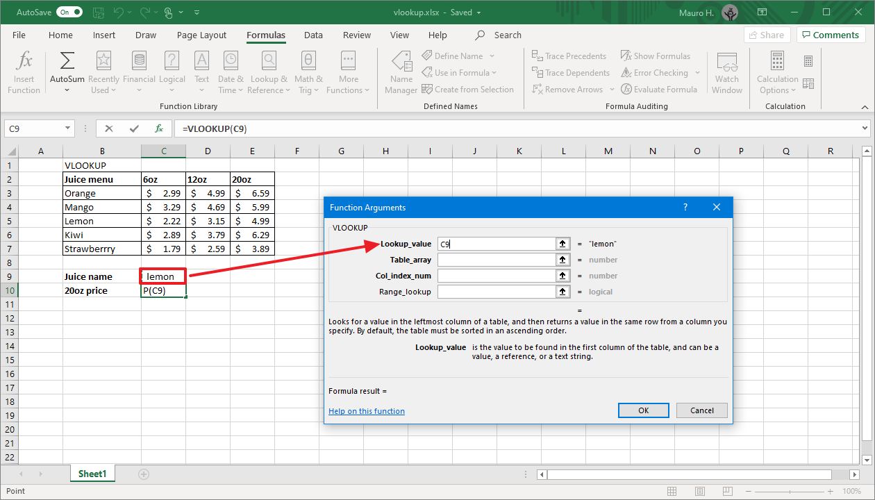
In the Lookup_value field, specify the cell that contains the reference of the item you want to find the answer to—for case, C9.

Source: Windows Central
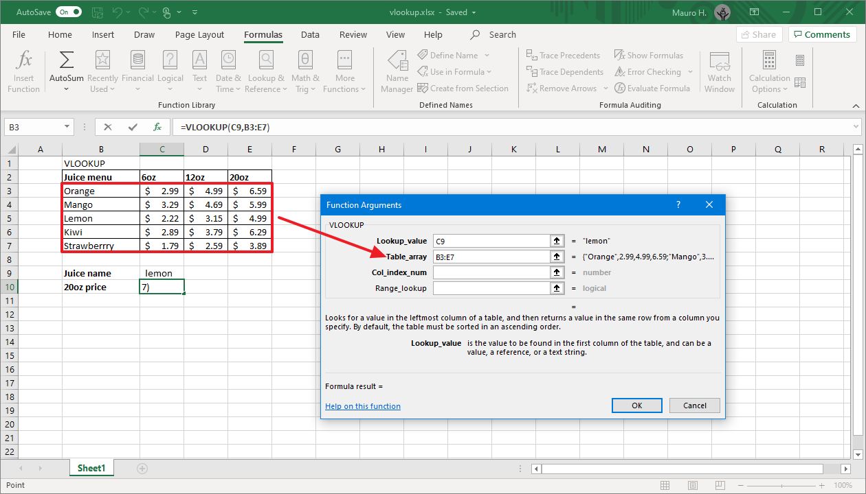
In the Table_array field, select the section of the table where the search will be performed. Usually, you want to select the unabridged table.

Source: Windows Key
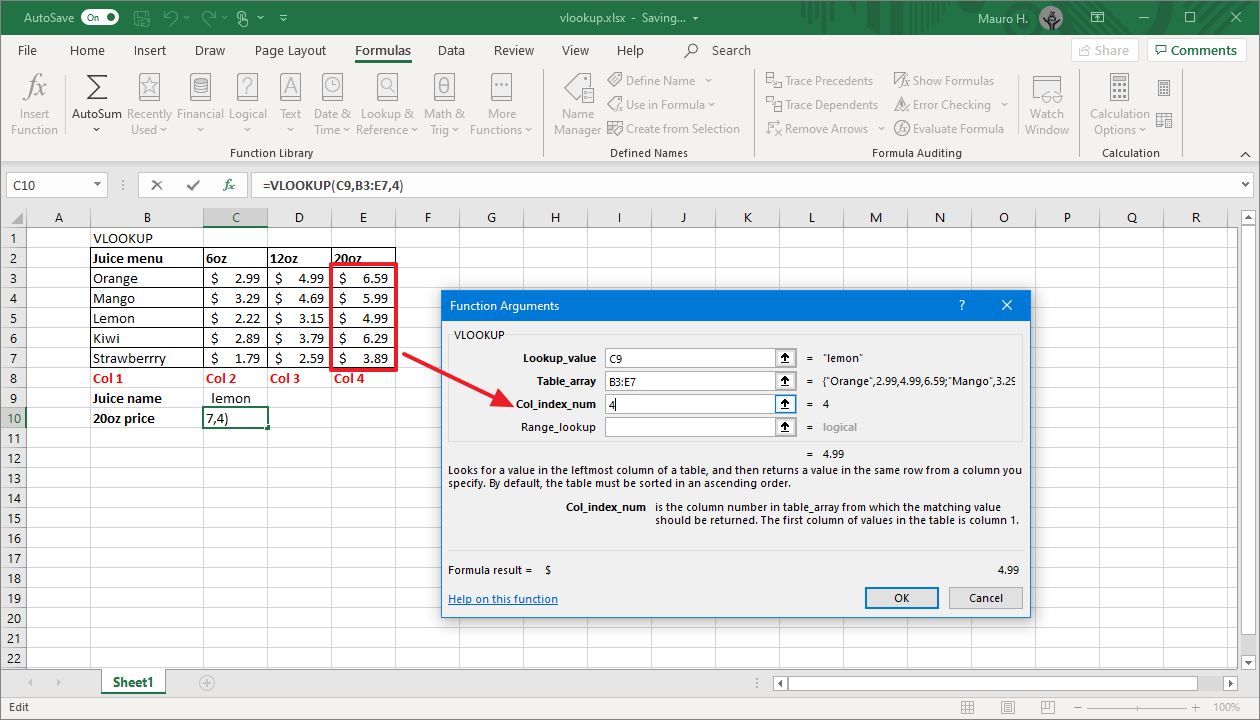
In the Col_index_num field, specify the cavalcade number that contains the respond. For case, 4, which is the number of the cavalcade that stores the data you want to call up. In this case, the cost for the 20oz bottle of juice.

Source: Windows Central
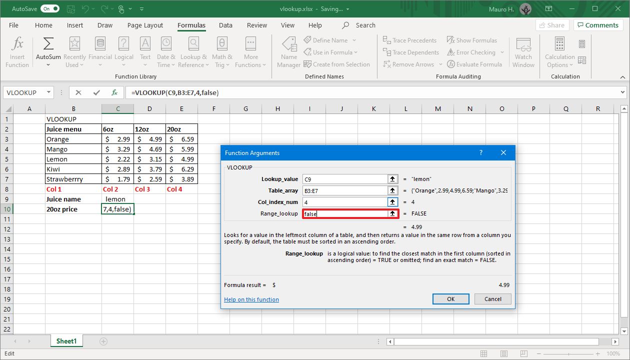
In the Range_lookup field, specify whether VLOOKUP should look for a specific match (false) or an approximate match (true).

Source: Windows Fundamental

Quick note: Typically, you desire to employ the false choice to query a specific match of the information you need.
Click the OK button.

After you complete the steps, VLOOKUP volition return the upshot based on the parameters you accept defined in the Function Arguments wizard.

In the instance that you want to decide the information for another particular with different details from the kickoff column, y'all desire to repeat steps No. four through 12.

We're focusing this guide on the desktop version of Microsoft Excel for Windows 10, simply yous can likewise employ VLOOKUP on the spider web version of Excel. However, the office magician is available, which ways you'll demand to write the formula manually with the above steps. Also, these instructions should work with the version of Office bachelor for macOS users.

More Windows 10 resources

For more helpful articles, coverage, and answers to common questions about Windows ten, visit the following resources:

Windows 10 on Windows Central – All you lot demand to know
Windows 10 help, tips, and tricks
Windows 10 forums on Windows Central

We may earn a commission for purchases using our links. Larn more.

An internet connection will soon be required when setting up Windows 11 Pro

UH OH

An internet connectedness volition soon be required when setting up Windows 11 Pro

Microsoft has announced that later this twelvemonth, users will be required to connect to the internet and sign-in with a Microsoft Account during the out of box setup experience on Windows 11 Pro. Microsoft has already been enforcing this requirement on Windows 11 Domicile since launch terminal Oct, and Windows xi Pro is now expected to follow suit soon.